Hey
多元线性回归问题
代价函数(整体数据集),损失函数(对于每个数据的误差)
learning_rate(从小的尝试比如0.0006)
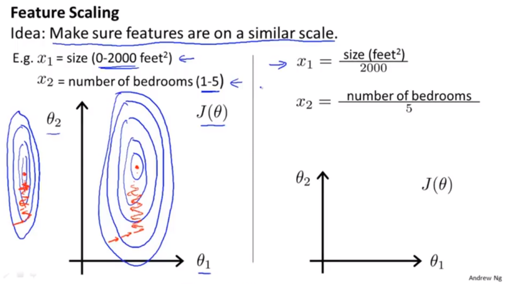
scaling the features(特征缩放)—适用与梯度下降改进 -Mean normalization(均值归一化)
- min-max标准化
X(每个数据) - U(特征值均值))/(Max-Min)
- Z-score标准化方法
X(每个数据) - U(特征值均值))/(std)
- 归一化
把数据变成(0,1)或者(1,1)之间的小数。主要是为了数据处理方便提出来的,把数据映射到0~1范围之内处理,更加便捷快速
normal equation(正规方程) or Gradient Descent
- normal equation is suitable for samll features(计算量比较大)
- Gradient descent is suitable for a large number for features(
 )
)
但是受数据的影响较大,所以对与Gradient descent来说需要进行feature scaling) normalize equation(正规方程)的公式推导
代价函数
矩阵不可逆:
1.矩阵存在线性相关的特征之值
2.矩阵所对应的行列式为0
homework(python)
1
2
3
4
5
6
7
8
9
10
11
12
13
14
15
16
17
18
19
20
21
22
23
24
25
26
27
28
29
30
31
32
33
34
35
36
37
38
39
40
41
42
43
44
45
46
47
48
49
50
51
52
53
54
55
56
57
58
59
60
61
62
63
64
65
66
67
68
69
70
71
72
73
74
75
76
77
78
79
80
81
82
83
84
85
86
87
88
89
90
91
92
93
94
95
96
97
98
99
100
101
102
103
104
105
import numpy as np
import matplotlib.pyplot as plt
import pandas as pd
from mpl_toolkits.mplot3d import Axes3D
data = pd.read_table("ex1data1.txt", header=None, delimiter=",", encoding="gb2312")
m = len(data)
data_x = np.array(data)[:, 0].reshape(m, 1)
data_y = np.array(data)[:, 1].reshape(m, 1)
# the first task
print(np.eye(5))
# the second task
# plt.scatter(data_x, data_y, color='r', marker='x',label="Training Data")
# plt.ylabel('Profit in $10,000s')
# plt.xlabel('Population of City in 10,000s')
# plt.show()
# the third task
def computeCost(X, y, theta):
inner = np.power(((X * theta) - y), 2)
return np.sum(inner / (2 * len(X)))
def gradientDescent(X,y,theta,alpha,epoch):
cost = np.zeros(epoch)
m = X.shape[0]
for i in range(epoch):
temp = theta - (alpha / m) * ((X * theta - y).T * X).T
theta = temp
cost[i] = computeCost(X,y,theta)
return theta,cost
def normal_equations(X,y):
theta = np.linalg.inv(X.T*X)*X.T*y
return theta
X = np.matrix(np.concatenate((np.ones((m, 1)), data_x), axis=1))
y = np.matrix(data_y)
theta = np.matrix(np.zeros([2, 1]))
alpha = 0.01
epoch = 1000
final_theta,cost = gradientDescent(X,y,theta,alpha,epoch)
print(final_theta)
final_theta = normal_equations(X,y)
print(final_theta)
x = np.array(list(data_x[:,0]))
f = final_theta[0,0] + final_theta[1,0] * x
# plt.scatter(data_x, data_y, color='r', marker='x',label="Training Data")
# plt.ylabel('Profit in $10,000s')
# plt.xlabel('Population of City in 10,000s')
# plt.plot(x,f,label="Prediction")
# plt.legend()
# plt.show()
# plt.plot(np.arange(epoch),cost,'r')
# plt.xlabel("Iteration")
# plt.ylabel("Cost")
# plt.show()
theta0_vals = np.linspace(-10,10,100)
theta1_vals = np.linspace(-1,4,100)
J_vals = np.zeros((len(theta0_vals),len(theta1_vals)))
for i in range(len(theta0_vals)):
for j in range(len(theta1_vals)):
t = np.matrix(np.array([theta0_vals[i],theta1_vals[j]]).reshape((2,1)))
J_vals[i,j] = computeCost(X,y,t)
######################################## 3D图 #######################################
# fig = plt.figure()
# ax = Axes3D(fig)
# ax.plot_surface(theta0_vals,theta1_vals,J_vals,rstride=1,cstride=1,cmap="rainbow")
# plt.xlabel('theta_0')
# plt.ylabel('theta_1')
# plt.show()
######################################## 3D图 #######################################
######################################## 等高线图 #######################################
# plt.figure()
# plt.contourf(theta0_vals, theta1_vals, J_vals, 20, alpha = 0.6, cmap = plt.cm.hot)
# a = plt.contour(theta0_vals, theta1_vals, J_vals, colors = 'black')
# plt.clabel(a,inline=1,fontsize=10)
# plt.plot(theta[0,0],theta[1,0],'r',marker='x')
# plt.show()
######################################## 等高线图 #######################################
data2 = pd.read_table("ex1data2.txt", header=None, delimiter=",", encoding="gb2312")
data2 = (data2 - data2.mean()) / data2.std()
m = len(data2)
data_x = np.array(data2)[:, 0:2].reshape(m, 2)
data_y = np.array(data2)[:, 2].reshape(m, 1)
data_x = np.concatenate((np.zeros((m,1)),data_x),axis=1)
X = np.matrix(data_x)
y = np.matrix(data_y)
theta = np.matrix(np.zeros((3,1)))
final_theta,cost = gradientDescent(X,y,theta,alpha,epoch)
plt.plot(np.arange(epoch),cost,'r')
plt.show()